
Initially big data started with collecting huge volume of data and processing it in smaller and regular batches using distributed computing frameworks such as Apache Spark. Changing business requirements needed to produce results within minutes or even in seconds.
This requirement is achieved by running the jobs in smaller interval (micro-batch) as per the result duration. There are various problems that arise with smaller intervals e.g. whether to process all data, which is inefficient, to produce result or does incremental processing and add the new result with the earlier results. How to ensure that records within an interval are available when the job is scheduled? Similarly, what to do if earlier job is still running when scheduling a new job. Stream processing framework solves such problems and provides the facilities for:
- Taking care of scheduling jobs, handling job failures and restart from the point of failure, similar to batch processing framework.
- Maintaining intermediate results and combine the results of previous batches to the current batch.
- Tracking if the previous batch is still running and waits for the completion before starting new batch.
- Providing facilities for unique streaming problems like late arrival of data records.
Stream processing is the superset of batch processing techniques. Spark extends batch processing APIs (Dataframe APIs) for stream processing.
Spark Structured Streaming
Spark introduced the idea of micro-batch processing. Data is collected for short duration, processing happens as micro-batch and output is produced. This process repeats indefinitely. Spark streaming framework takes care of the following:
- Automatic looping between micro batches
- Batch start and end position management
- Intermediate state management
- Combining results to the previous batch results
- Fault tolerance and restart management
Spark streaming was initially supported using DStream APIs, which are based on RDD. Since these are based on RDD**, it does not take advantage of *Spark SQL engine optimization. It also does not support Event Time Semantics. No further enhancement and upgrades are expected for DStream APIs.
An enhanced version of Spark Streaming is now supported, called Structured Streaming APIs, which is based on Dataframe APIs. It provides unified model for batch and stream processing. Being based on Dataframe APIs, it takes advantage of Spark SQL engine optimization. It also supports Event Time Semantics.
Spark Stream Processing Model
Spark stream processing query runs as micro-batches. Each micro-batch starts with a new input Dataset, process it and writes the data to the Spark Sink. Next micro-batch starts with another new input Dataset and this all goes on in a loop. All of this is internally managed by a background thread. There is no loop in the application written. Starting a query acts like an Action. Spark driver takes the code starting from the Read Stream until the Write Stream and submits it to Spark SQL engine, which compiles and optimizes the code and generate an execution plan. Execution plan is then executed using a background thread, which run micro-batch jobs.
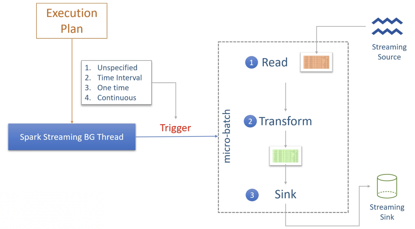
Each micro-batch job and data is determined by the Trigger. Following are the supported trigger types:
- Unspecified — is the default trigger and starts a new micro-batch as soon as the current micro-batch processing is over and data is available.
- Time Interval — sets time limit for each micro-batch. Only after the interval specified is passed, next micro-batch may start. It takes care of not starting new micro-batch until the current one is over even though current micro-batch has exceeded its time.
- One Time — is like a batch processing. It triggers only one job and then background process stops.
- Continuous — is an experimental feature to provide millisecond latency.
Spark Streaming Sources
Spark allows four built-in sources:
- Socket Source allows to read data from a socket source. It is generally not used in production.
- Rate Source is a dummy data source which generates configured number of (key, value) pairs per second. It is used for testing and benchmarking application.
- File Source reads from files at a specified location. Number of files processed in a micro-batch is based on the configuration. Spark Streaming framework provides exactly-once processing, wherein each record is processed exactly one time. readStream is used to read a file stream to get streaming Dataframe instead of read method to read a single file to get standard Dataframe. File source is used where trigger can be in minutes.
- Kafka Source is useful for low latency stream processing application which require processing in seconds or less than a second.
Spark Streaming Sinks
Similar to streaming Sources, Spark Streaming has built-in support for a number of streaming data sinks (for example, files and Kafka) and programmatic interfaces that allow to specify arbitrary data writers.
Spark Streaming Output Modes
There are three output modes:
- Append mode is an insert only operation. Previous output records are not updated and each micro-batch writes new records only.
- Update is like upsert operation. Output records contains either new or old records that are updated.
- Complete is similar to overwrite operation. Previous records are overwritten with the new records.
Checkpoint, fault Tolerance and restart
A stream processing application in Apache Spark is expected to be running an infinite loop of micro-batches. But application may stop either due to failure or scheduled maintenance (upgrade). In such scenario, application should restart while maintaining the exactly-once semantics i.e.
- Do not miss any input records
- Do not create duplicate output records
This is achieved by maintaining state (read position, state information) of micro-batches in checkpoint location. Checkpoint information is enough for restarting a unfinished micro-batch but this does not guarantees exactly-once requirements which needs:
- Restart with same checkpoint location — this is basic requirement. If checkpoint directory is deleted or query is started with a new location, it is going to be a new query.
- Replay-able data Source — file and Kafka data source allows to replay the data from a specific time. However, Socket data source does not allow to replay the data.
- Deterministic computation — application logic should produce the same result given the same input data. In case application logic is using current date or time based logic, the output for the same input data will be different based as data and time keeps changing.
- Idempotent Sink — output sink should be able to identify duplicates, ignore them or update the older copy of the same record.
In case of bug fixes, application code will be changed. Spark allows code changes and restart from the same checkpoint information as long as changes does not cause conflict with checkpoint information.
Windowing and Aggregates
Spark streaming transformation are broadly classified as:
- Stateless Transformations
- Stateful Transformations
This classification is with respect to the data maintained in state store, which is stored by micro-batch job to be used for future reference by later micro-batch jobs. All the projection transformations such as select, filter, map, flatmap, explode are stateless transformations as they do not need to maintain states across the micro-batches. Grouping, aggregation, windowing and joins transformation are stateful transformations because they need to maintain states across the micro-batches.
Stateful transformation does not support the complete output mode as these queries produce one or more record for each input record that does not depend on previous queries. On the other hand, excessive state for stateful transformation may cause out of memory issues as the state is cached in executors memory. State is check-pointed and saved in check point location, which is used to restart the application in case of a failure. Time-bound state should be used so that Spark can clear the outdated states. If time-bound state is not possible, you should use unmanaged stateful transformation and provide custom cleanup logic.
The time-bound aggregations are computed for specific time window. These time-bound aggregates are also known as windowing aggregates. These time windows are of two types: Tumbling Window and Sliding Window.
Tumbling Window
In a tumbling window, events are grouped in a single window based on time. An events belongs to only one window.
For example, consider a time-based tumbling window with a length of five seconds. The first window (w1) contains events that arrived between the zeroth and fifth seconds. The second window (w2) contains events that arrived between the fifth and tenth seconds, and the third window (w3) contains events that arrived between tenth and fifteenth seconds. The tumbling window is evaluated every five seconds, and none of the windows overlap; each segment represents a distinct time segment.

An example would be to compute the average price of a stock over the last five minutes, computed every five minutes.
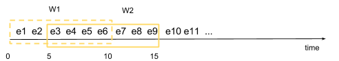
Sliding Window
In a sliding window, events are grouped within a window that slides across the data stream according to a specified interval. Sliding windows can contain overlapping data; an event can belong to more than one sliding window.
In the following image, a time-based sliding window with a length of ten seconds and a sliding interval of five seconds is used. The set of events within the window are evaluated every five seconds. The first window (w1) contains events that arrived between the zeroth and tenth seconds. The second window (w2) contains events that arrived between the fifth and fifteenth seconds. Note that events e3 through e6 are in both windows. When window w2 is evaluated at time t = 15 seconds, events e1 and e2 are dropped from the event queue.
An example would be to compute the moving average of a stock price across the last five minutes, triggered every second.
Watermarks
Watermark can be considered as a threshold for how long to wait for late arrival of data. Generally, data is processed asynchronously and sent across a network. It is highly likely that data may arrive out of order or not at all. Spark streaming provides an option to specify event time to base the watermark off. Spark handles buffering the data and computations to be performed for the duration specified as the watermark.
Watermark can be enabled by simply adding the withWatermark-Operator to a query:
withWatermark(eventTime: String, delayThreshold: String): Dataset[T]
It takes two Parameters,
- an event time column (must be the same as the aggregate is working on) and
- a threshold to specify for how long late data should be processed (in event time unit).
The state of an aggregate will then be maintained by Spark until max eventTime — delayThreshold > T, where max eventTime is the latest event time seen by the engine and T is the starting time of a window.
Joins
Structured streaming supports two types of joins:
- Streaming Dataframe to Static Dataframe
- Streaming Dataframe to Streaming Dataframe
Streaming Dataframe is joined to Static Dataframe for stream enrichment. For example, if a stream is coming for a user (based on userID), you may like to get information about the user from a static table (e.g. userName). This operation is stateless as one side of the join is fully known (Static Dataframe).
Streaming Dataframe to Streaming Dataframe is a stateful operation. Spark buffers both sides of data in state store and keeps checking it as new data arrives. Without specifying a watermark on the join, Spark will buffer the state of each of the two streams… indefinitely!
The watermarks let Spark know how long data can be delayed, for each Spark Dataframe being joined. Watermark need to be applied to both the stream, though the value of watermark may be different between streams.
References
- Apache Spark 3 — Real-time Stream Processing using Python — Udemy, Prashant Kumar Pandey
- Tumbling vs Sliding Window